An inequality measure is often a function that ascribes a value to a specific distribution of income in a way that allows direct and objective comparisons across different distributions. To do this, inequality measures should have specific properties and behave in a certain way given certain events. For example, moving $1 from a richer person to a poorer person should lead to a lower level of inequality. No single measure can satisfy all properties, though, so choosing one measure over another involves trade-offs. The following measures differ with regard to the properties they satisfy and the information they present. None can be considered superior, as all are useful in specific contexts. A well-balanced analysis of inequality should look at several of these measures.

In this post, I teach to compute three indexes of income inequality using data from the 2016 Census of Population [Canada], the Public Use Microdata File (PUMF).

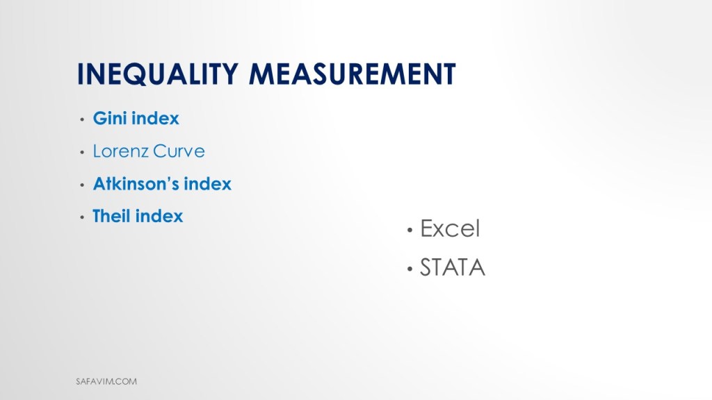
The Lorenz curve is the first one. Other indexes discussed here include the Gini, Atkinson, and Theil indices.

DATA
Canadian Income Survey, 2016 (CIS 2016)
Income data has been used extensively by researchers to better understand the economic well-being of Canadians. To meet the needs of these users, Statistics Canada has produced numerous cross-sectional public use microdata files (PUMFs). The CIS is a cross-sectional survey developed to provide information on the income and income sources of Canadians, with their individual and household characteristics. It is a short questionnaire asking a sub-sample of respondents to the Labor Force Survey (LFS), gathering information on labor market activity, school attendance, support payments, child care expenses, inter-household transfers, personal income, and characteristics and costs of housing. The CIS content is supplemented with information from the LFS on individual and household characteristics (e.g., age, educational attainment, main job characteristics, and family type) and with tax data for income and income sources (Statistics Canada, 2016a).

Universe
The target population of CIS is all individuals in Canada, excluding residents of the Yukon, the Northwest Territories, and Nunavut, residents of institutions, persons living on reserves and other Aboriginal settlements in the provinces, and members of the Canadian Forces living in military camps. Overall, these exclusions amount to less than 3 percent of the population.

Sampling Procedure
The CIS sample is a sub-sample of the Labour Force Survey sample. LFS uses a complex random sampling plan to select the households. Each household in the sample represents several other households in the population. Estimates for a given characteristic are obtained by multiplying the survey weight by the corresponding value of this characteristic. The key step in the point estimation process is, therefore, the derivation of the weight.
The initial weights are the LFS sub-weights, which are then adjusted to account for the fact that the CIS is a sub-sample of the LFS sample.
It is the responsibility of data users to apply the weights for any estimates they wish to produce. If weights are not used, the results derived from the microdata cannot be considered to be representative of the survey population. On the CIS PUMF file, the weight variable is named FWEIGHT (Income Reference Guide, Census of Population, 2016, n.d.).

The 2016 Census public use microdata file (PUMF) on individuals contains 930,421 records, representing 2.7% of the Canadian population.

Variables

•Total Income: It is referred to as income before transfers and taxes.

•Market Income: It is equivalent to total income minus government transfers.

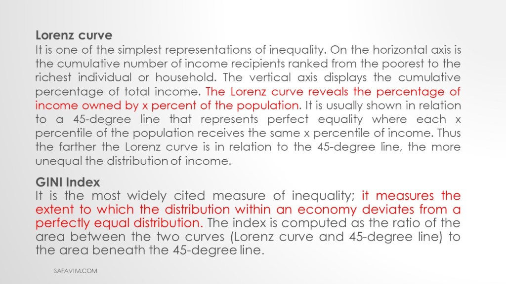
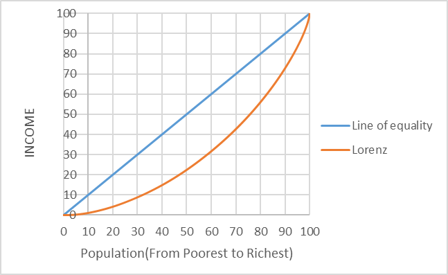
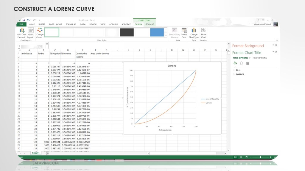
Lorentz curve
It is among the simplest ways to illustrate inequality. The total number of income recipients, ranked from the poorest to the richest person or household, is shown on the horizontal axis. The cumulative percentage of total income is represented on the vertical axis. The Lorenz curve shows what proportion of the population owns what percentage of income. It is frequently depicted in relation to a 45-degree line that represents perfect equality, in which each individual in the xth percentile of the population receives an income at the xth percentile. Therefore, the distribution of income is more unequal the farther the Lorenz curve is from the 45-degree line.

GINI Index
It measures how far the distribution within an economy deviates from a perfectly equal distribution and is the most frequently used indicator of inequality. The area between the two curves—the Lorenz curve and the 45-degree line—to the area below the 45-degree line is used to calculate the index.

Measuring GINI using Excel

To start measuring income inequality, open a new sheet in excel.

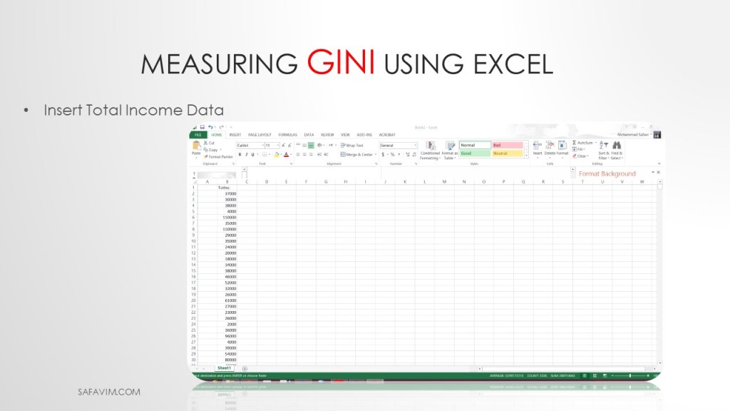
In the next step, insert data into the spreadsheet.

Sort data from smallest to largest.

Insert Individual Number in a column.

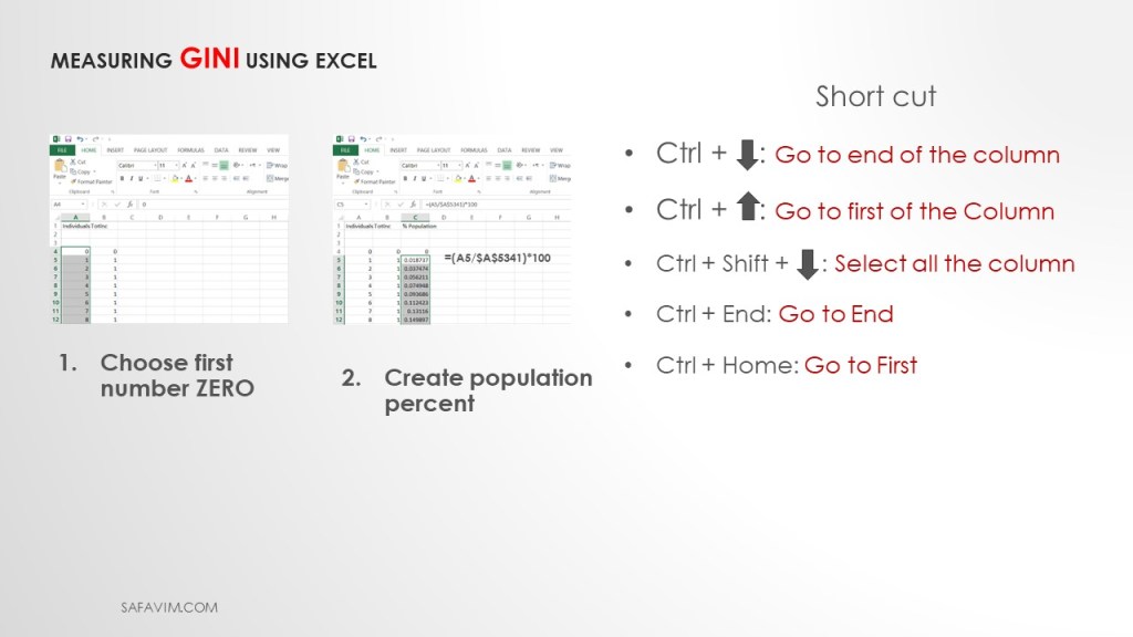
Using this formula (=(A5/$A$5341)*100) create population percent in column C

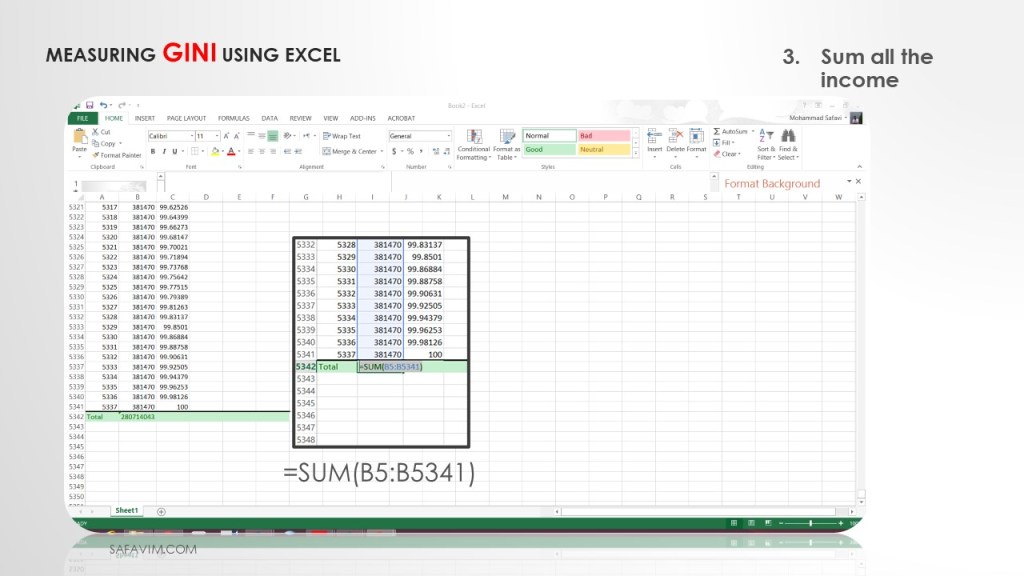
Using this formula (=SUM(B5:B5341), sum all the income in the last row of column B.

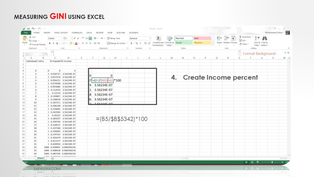
Using this formula ( =(B5/$B$5342)*100), create income percent in column D.

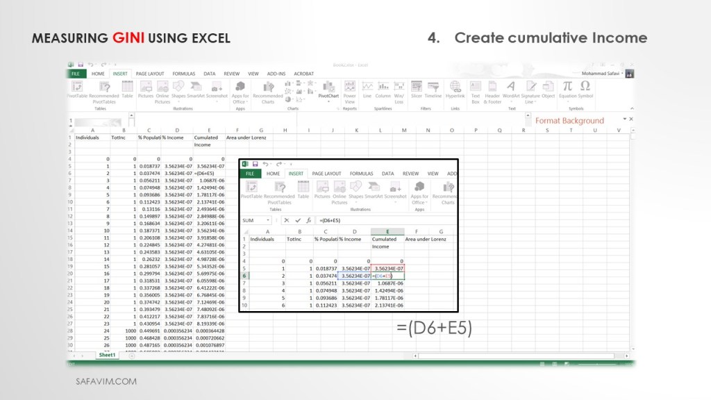
Create cumulative income in Column E using this formula (=(D6+E5)) as shown in picture 13.

As shown in picture 14, draw a Scatter Smooth line using the menu.

Select data and add to Scatter Smooth Line.

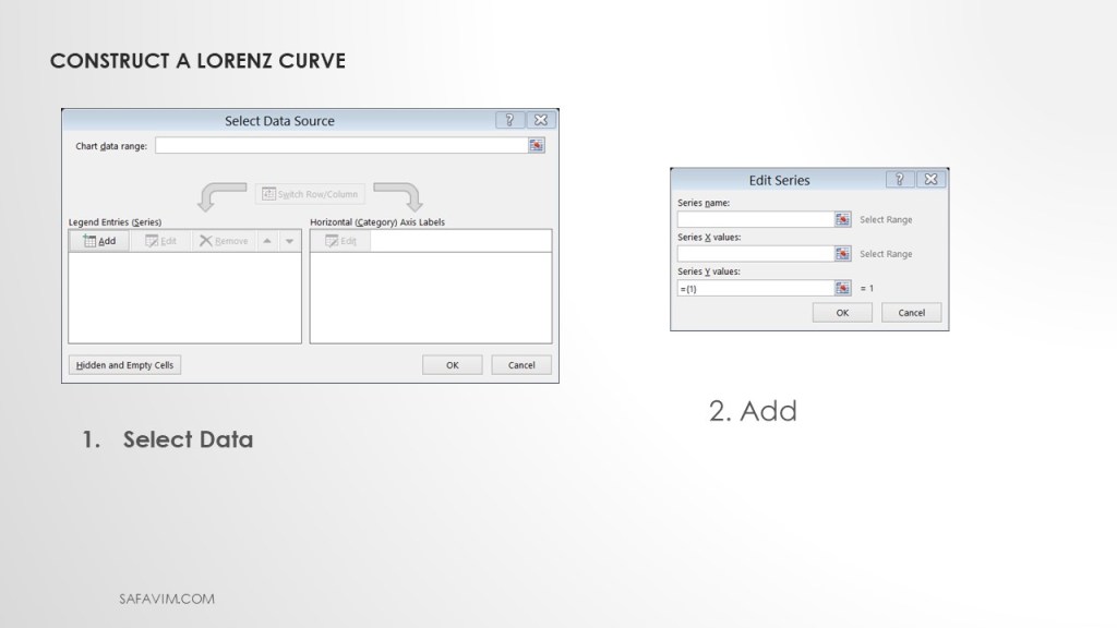
To Create the Line of Equity, In the Edit Series window, using the short cut follow these steps:
1- Series Name: Line of Equality
2- X-Axis: Select all Data – Percent Population
3- Y-Axis: Select all Data – Percent Population

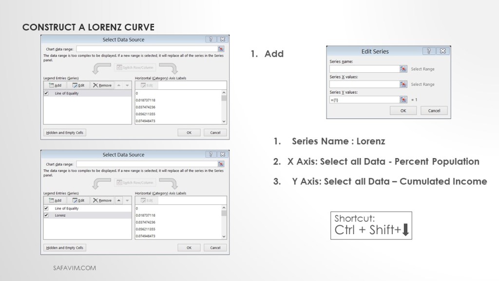
To construct the Lorenz curve, In the Edit Series window, using the short cut follow these steps:
1- Series Name : Lorenz
2- X-Axis: Select all Data – Percent Population
3- Y-Axis: Select all Data – Cumulated Income

Now we want to compute the GINI index.

To calculate the GINI index, we need to calculate the area under the Lorenz curve.

In each rectangle in this area, under the Lorenz curve, we must sum the boundary of the bottom and the upper bound of the cumulative income and divide it by two. (The mean of the high bound and the low bound of each rectangle).

Then we need to multiply by the width of each rectangle.

Using this formula (=((E5+E4)/2)*0.018737118231216))), we can calculate the area under the Lorenz curve.

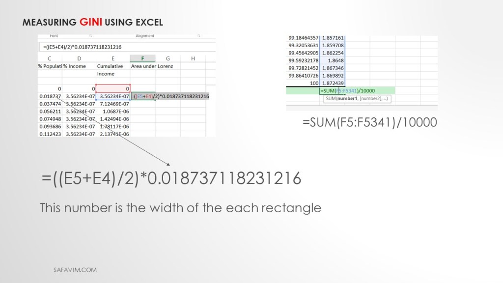
As picture 20 shows, each cell of column C is the width of each rectangle.

In the next step, we need to sum up column F to calculate the area under the Lorenz curve. (=SUM(F5:F5341)/10000)

As picture 21 shows, using these two formula we can calculate the GINI index. 1- (=0.5-F5342) 2- (=J31/0.5)

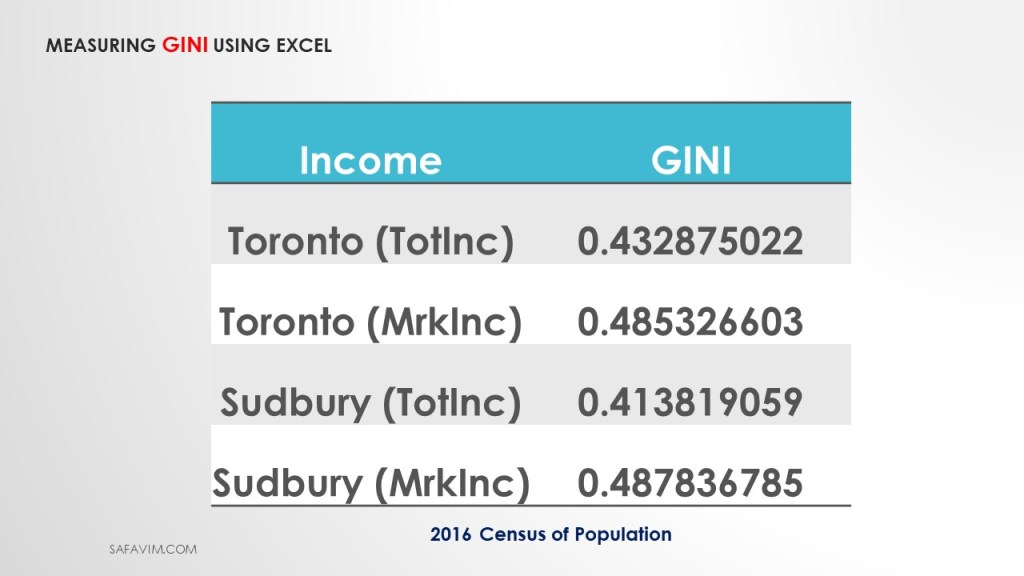
As shown in picture 23, four different Gini indexes were measured using Total income and Market income.

We continue to measure the Gini index using STATA.

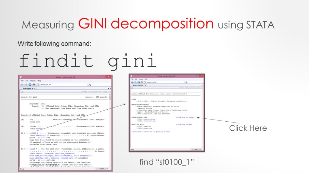
We need to install the Gini package in Stata. To do that write follwing command.

findit gini

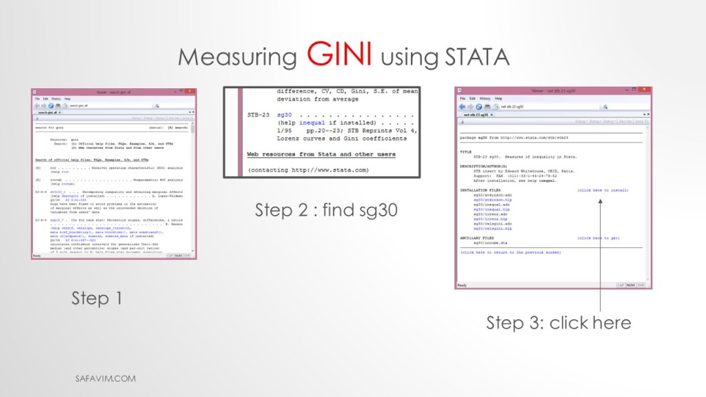
As picture 26 shows, do three steps to install the package.

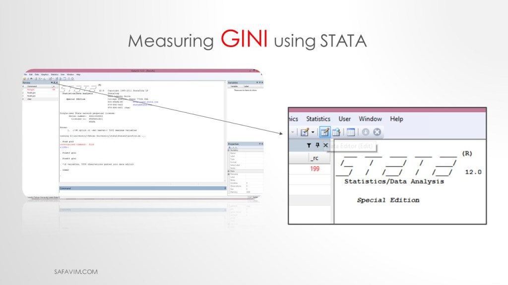
Copy data from Excel to Stata.

Pictures 27 and 28 show the pathway to copy the data from Excell to Stata.

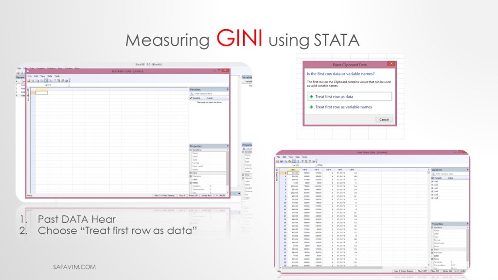
Follow two steps here. 1- Past DATA Hear 2- Choose “Treat first row as data”

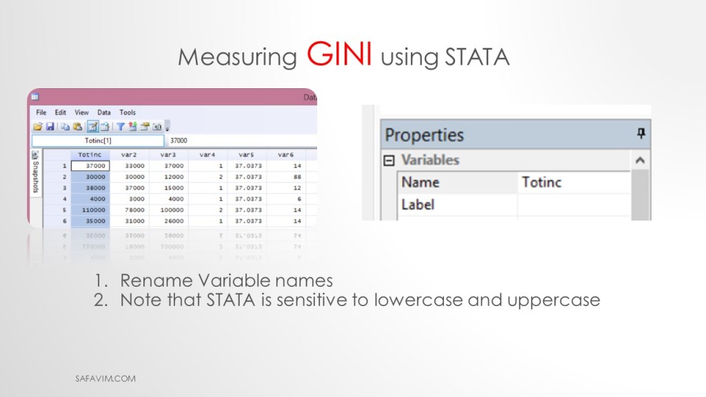
1- Rename Variable names
2- Note that STATA is sensitive to lowercase and uppercase.

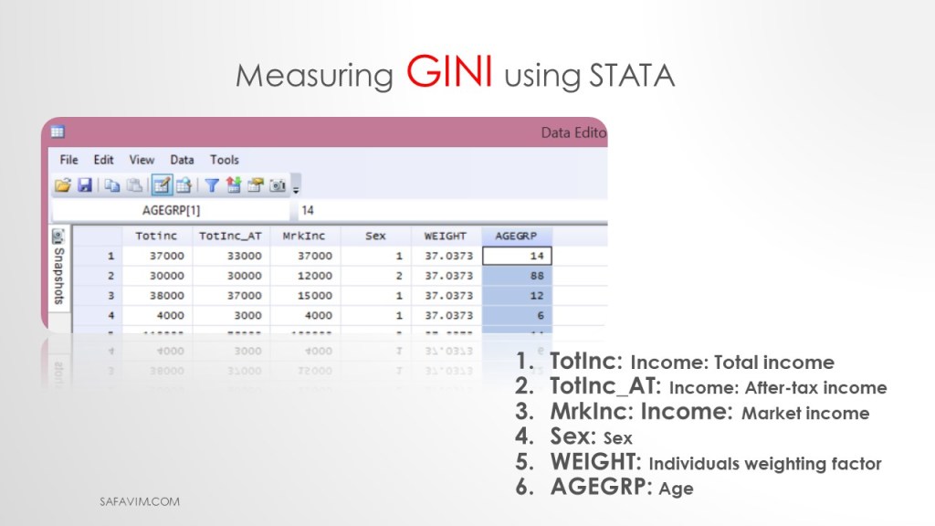
TotInc: Income: Total income
TotInc_AT: Income: After-tax income
MrkInc: Income: Market income
Sex: Sex
WEIGHT: Individual weighting factor
AGEGRP: Age

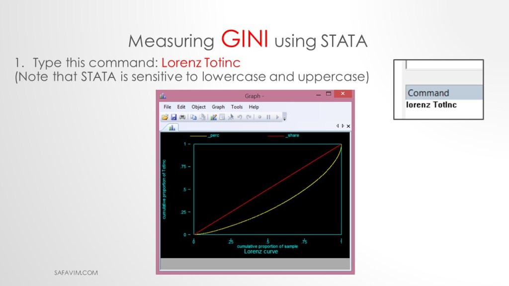
Using the following command, we can draw the Lorenz curve in Stata.

1- Type this command: Lorenz Totinc
2- Note that STATA is sensitive to lowercase and uppercase

Using the following command, we can calculate Gini in Stata.

1- Type this command: inequal Totinc
2- (Note that STATA is sensitive to lowercase and uppercase)

Usind the following command we can see the help in Stata.

help inequal

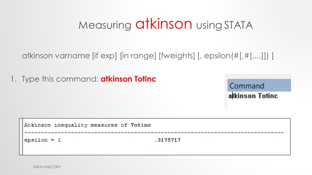
Using the following command, we can calculate Atkinson index in Stata.

Type this command: atkinson Totinc

This is the general command:

atkinson varname [if exp] [in range] [fweights] [, epsilon(#[,#[,…]]) ]

The Gini coefficient is widely used to measure inequality in the distribution of income, wealth, expenditures, etc. We can comprehend the causes of inequality better by decomposing this measure.

Now we want to decompose the Gini index. Follow the steps in picture 36 to install the Gini package.

To see help decomposition, write the command below.

help descogini

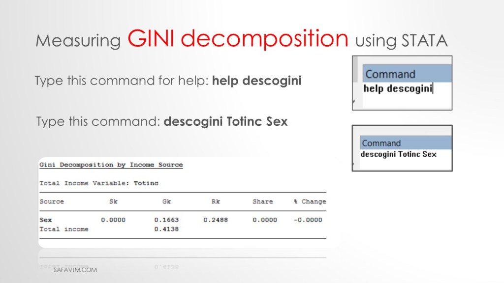
Type this command: descogini Totinc Sex

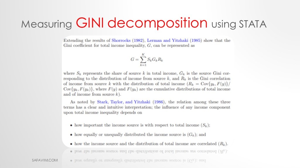
Lerman and Yitzhaki (1985) show that the Gini coefficient for total income, G, can be represented as:

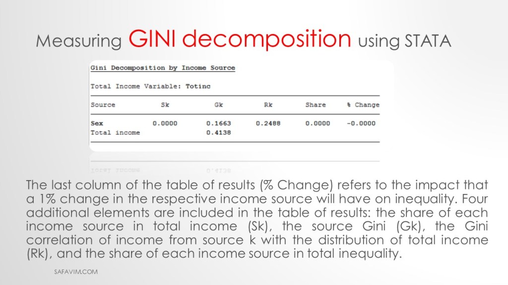
As can be seen in picture 40, the last column of the table of results (% Change) refers to the impact that a 1% change in the respective income source will have on inequality.

Four additional elements are included in the table of results:

the share of each income source in total income (Sk),

the source Gini (Gk),

the Gini correlation of income from source k with the distribution of total income (Rk),

and the share of each income source in total inequality.

Measuring Inequality indices, with decomposition by subgroup using STATA.

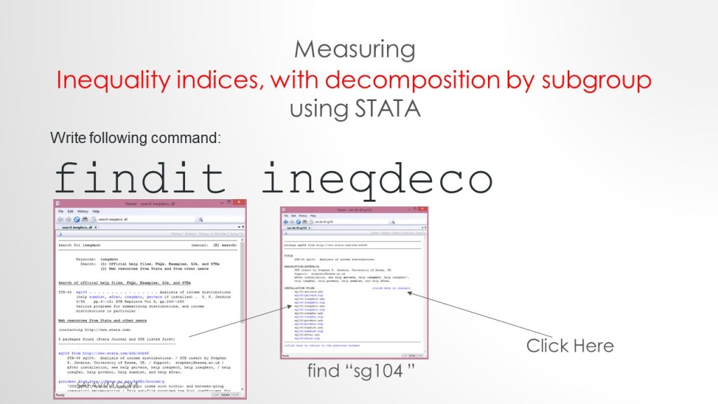
Follow the steps in picture 41 to install syntax on Stata.

findit ineadeco

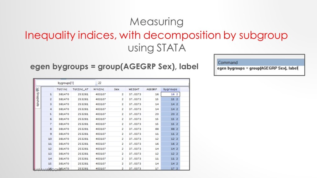
Use the following syntax to create the group.

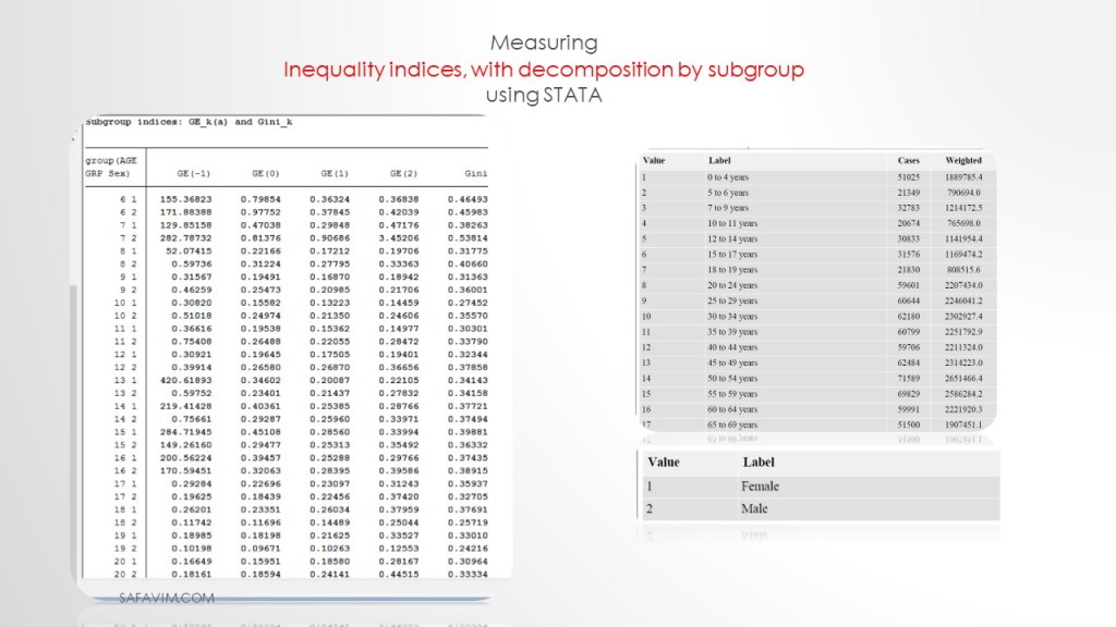
egenbygroups = group(AGEGRP Sex), label

“ineqdeco” estimates a range of inequality and related indices commonly used by economists, plus decompositions of a subset of these indices by population subgroup. Inequality decompositions by subgroup are helpful in providing inequality profiles’ at a point in time and for analyzing secular trends using shift-share analysis. Unit record (micro’ level) data are required.

Use following syntax to run the command.

ineqdeco Totinc, by(bygroups)

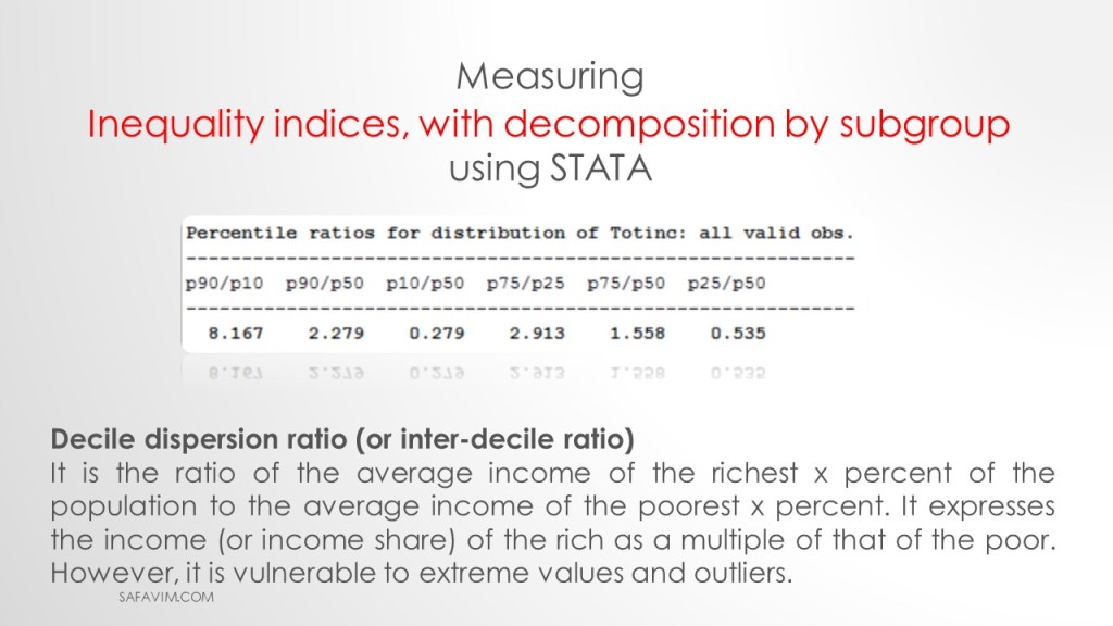
Decile dispersion ratio (or inter-decile ratio)
It is the ratio of the average income of the richest x percent of the population to the average income of the poorest x percent. It expresses the income (or income share) of the rich as a multiple of that of the poor. However, it is vulnerable to extreme values and outliers.

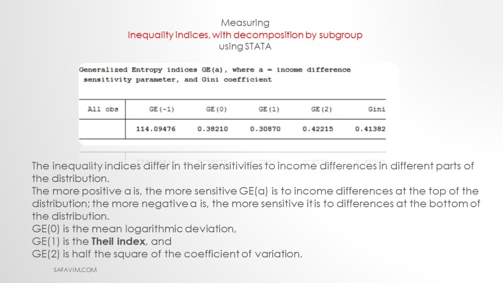
The inequality indices differ in their sensitivities to income differences in different parts of the distribution.
The more positive a is, the more sensitive GE(a) is to income differences at the top of the distribution; the more negative a is, the more sensitive it is to differences at the bottom of the distribution.
GE(0) is the mean logarithmic deviation,
GE(1) is the Theil index, and
GE(2) is half the square of the coefficient of variation.

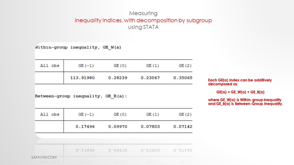
Each GE(a) index can be additively decomposed as

    GE(a) = GE_W(a) + GE_B(a)

where GE_W(a) is Within-group Inequality and GE_B(a) is Between-Group Inequality.

Reference

Income Reference Guide, Census of Population, 2016. (n.d.). Retrieved January 30, 2023, from https://www12.statcan.gc.ca/census-recensement/2016/ref/guides/004/98-500-x2016004-eng.cfm

Lerman, R. I., & Yitzhaki, S. (1985). Income inequality effects by income source: A new approach and applications to the United States. The review of economics and statistics, 151-156.

Shorrocks, A. F. (1982). Inequality decomposition by factor components. Econometrica: Journal of the Econometric Society, 193-211.

#Gini #Theil #Income_inequality #Decomposition #decile_ratio #STATA #Excel